Submission

Submit your notebook here

---

Deliverable

Submit one notebook that includes:

1. Loaded protein_embeddings.pkl created in Route 36A
2. Implemented get_window_embedding(...) and tested it
3. Built reference-vs-sliding cosine similarity profile
4. Built full window-vs-window cosine heatmap
5. Wrote a short interpretation tied to UniProt annotations

Mission checklist

• Loaded generated embedding dictionary
• Extracted a window embedding
• Computed reference-vs-sliding cosine profile
• Plotted similarity profile with reference marker
• Computed full similarity matrix
• Plotted heatmap and interpreted biological signal

🧗 Summit

---

Exercise 4: Extra Credit Scale to More Proteins

1. Repeat Exercises 2-3 for at least 2 additional proteins
2. Compare qualitative heatmap patterns across proteins
3. Add one hypothesis for why patterns differ biologically

🤸 Dyno up

---

Exercise 3: Full Cosine Heatmap Window vs Window

1. Pick the same protein you used in Exercise 2
2. Use window size 10
3. Precompute all window embeddings, then compute all pairwise cosine similarities
4. Plot heatmap:
   • X-axis: window start position
   • Y-axis: window start position
   • Color: cosine similarity
5. Interpret:
   • diagonal behavior
   • off-diagonal blocks/bands
   • one plausible link to UniProt domain/function notes

🦵 Heel hook up

---

Exercise 2: Reference vs Sliding Cosine Profile

1. Choose one protein from your dictionary (prefer L >= 120)
2. Set window_size = 5
3. Set ref_pos = L // 2
4. Compute cosine similarity between reference window and all valid sliding windows
5. Plot profile with a vertical line at ref_pos
6. Write 2-4 sentences interpreting the shape of the profile

🧱 Stem up

---

Exercise 1: Build Window Embedding Function

Implement:

get_window_embedding(emb_dict, uniprot_id, start_pos, window_size)

Requirements:

1. Slice [start_pos : start_pos + window_size]
2. Mean-pool residues in that slice
3. Return shape (1280,)

Required test:

• Pick one ID from your dictionary
• Use window_size = 5
• Use start_pos = min(50, L - window_size)
• Print shape and short preview values

🤚 Undercling up

---

Exercise 0: Load Embeddings from Route 36A

You must complete Route 36A first.

Load your generated file:

import pickle

with open("protein_embeddings.pkl", "rb") as f:
    emb_dict = pickle.load(f)

print(type(emb_dict), len(emb_dict))
for k in list(emb_dict.keys())[:3]:
    print(k, emb_dict[k].shape)

Checks:

1. Object is a dictionary
2. Multiple proteins are present (target 10-20)
3. Each value has shape (L, 1280)

If you do not have this file yet, complete Route 36A first.

🪢 Clip in

---

Intro

This route is the second half of the PLM practice final prep.

You already generated residue-level embeddings in 36A. Now you will analyze local regions by sliding windows and cosine similarity.

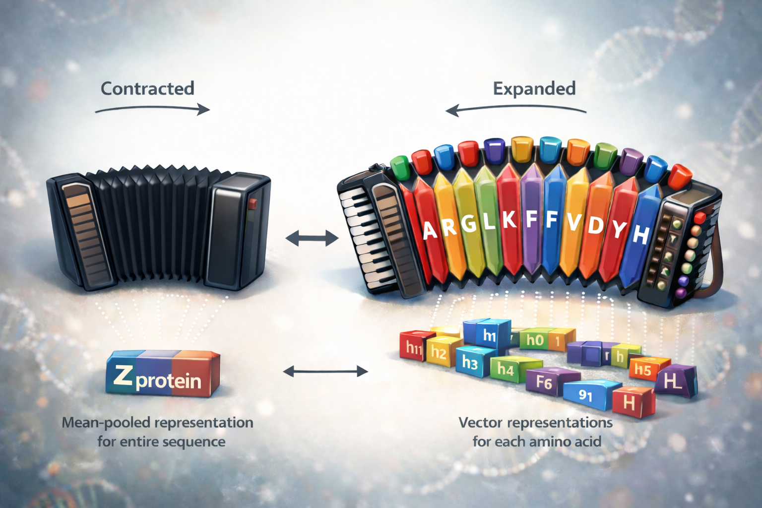
The core move is the accordion idea:

• residue embeddings are the expanded representation
• mean pooling contracts local windows
• cosine similarity compares local regions across the protein

💪 Mantle up

---

Route 036B: Residue-Level PLM Cosine Analysis

• RouteID: 036B
• Wall: Protein Representations (W05)
• Grade: 5.10a
• Routesetter: Course Staff
• Time: ~45-60 minutes
• You'll need: protein_embeddings.pkl from 36A, notebook runtime, plotting, and UniProt lookup.

🧗 Start climbing!